Welcome to our website. Our group, based in the Department of Chemistry and Materials Science at Aalto University, Finland is led as Principal Investigator by Prof. Miguel Caro. We carry out academic research on computer simulation of materials using atomistic models. Browse the website to find out more about our work.

Announcements and latest news


Three PhD student positions available in the groupJuly 4, 2025We have three vacant PhD student positions in the group. For more information and to apply (deadline 31 July 2025), check this website. [...]
Read more...
Experiment-driven computational simulation of materialsMay 22, 2024This is a synopsis of the paper by T. Zarrouk, R. Ibragimova, A.P. Bartók and M.A. Caro, “Experiment-Driven Atomistic Materials Modeling: A Case Study Combining X-Ray Photoelectron Spectroscopy and Machine Learning Potentials to Infer the Structure of Oxygen-Rich Amorphous Carbon”, J. Am. Chem. Soc., DOI:10.1021/jacs.4c01897, available as an Open Access PDF from the publisher’s website. All figures are reproduced under the CC-BY 4.0 license.
The atomistic modeling field is rapidly evolving in the midst of a machine learning (ML) and artificial intelligence (AI) driven revolution. Simulations of molecules and materials, involving thousands and even millions of atoms, or molecular dynamics (MD) simulations spanning long simulation times, are now routinely done with (close to) ab initio accuracy. These were unthinkable just a decade ago. Yet, the ultimate test for any theory and simulation is experiment, and achieving experimental agreement and incorporating experimental data directly into these atomistic simulations is necessarily the next frontier in atomistic modeling.
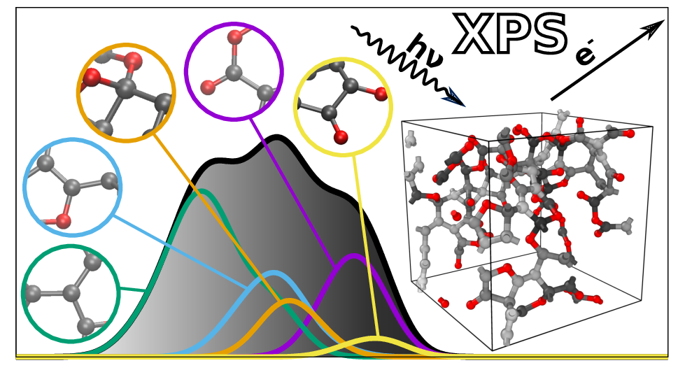
A central object of atomistic materials modeling is obtaining the atomic-scale structure of materials. This is particularly important (and interesting) when the material lacks crystalline ordering and experimental techniques like X-ray diffraction (XRD) cannot be used to determine its structure. Amorphous and generally disordered materials are one such class of materials, but also liquids and interfaces are relevant here. Through atomistic modeling we can attempt to derive structural models of these materials, e.g., a set of representative structures given in terms of the atomic positions (the Cartesian coordinates of the atoms). After deriving these models, we want to connect the simulation with the experiment, both to verify the soundness of the computational approach and to gain atomistic insight into the structure of the material. One of the different ways to do this, indirectly, is by using spectroscopy techniques, like X-ray photoelectron spectroscopy (XPS). On the one hand, we measure the XPS spectrum of the material experimentally; on the other, we make a computational XPS prediction for our candidate structural model. If they agree, we gain confidence that the model resembles reality; if they don’t, we keep looking for better structural models. (Of course, the whole story is more nuanced but this is the gist of it).
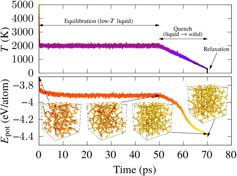
During our previous work on XPS prediction in collaboration with Dorothea Golze, we showed how XPS prediction for amorphous carbon-based materials can be made quantitatively accurate via a combination of electronic structure methods and atomistic machine learning technology. One of the disappointing aspects of that work is that we were unable to generate structural models of oxygenated amorphous carbon (a-COx) whose XPS spectra matched the experimental one. Since we had very good confidence in the accuracy of our computational XPS prediction, the necessary consequence was that the computational models of the structure of a-COx we were working with did not resemble the experimental samples. At the time, these models had been provided by our collaborator Volker Deringer from expensive DFT calculations, and we only had access to three a-COx models with a couple hundred atoms and different oxygen content. I was left intrigued by this issue and decided to train a machine learning potential (MLP) for CO. With this MLP, I could efficiently generate lots (thousands if not millions) of different samples at different conditions and thought: “surely, one of them will give the match with experiment”. But this was not the case! The reason is that the experimental growth is a non-equilibrium process involving energetic deposition of atoms: C atoms are deposited onto a growing film in an oxygen atmosphere, and the oxygen atoms are co-deposited with the carbon atoms into the film (see the nice work by Santini et al.). Direct simulation of the deposition process is very challenging. Our computational generation protocol was based on indirect structure generation routes and favored the formation of thermodynamically stable products: solids with low oxygen content and lots of CO and CO2 molecules.
“Regular” structure generation protocols failed to produce samples with computational XPS compatible with the experimental reference.
At this point, we had to think a bit outside the box. The idea that came to mind was something that is known in the literature as reverse Monte Carlo (RMC): the atomic positions are updated and the observable directly comparable to experiment is monitored on the fly, such that moves that increase the agreement between simulation and experiment for said observable are favored. After many steps, computational and experimental observables will agree. There are (at least) two problems with this approach, and both are related to the need for cheap calculations, given the sheer number of individual evalutations of the system’s energy required in Monte Carlo optimization. First, RMC for materials has traditionally been done using XRD only, because this is computationally cheap to compute given a set of atomic positions. Second, the RMC protocol will not ensure that the generated structures are energetically sound (low in energy) as the only constraint is that the agreement with the experimental observable should improve. Previous work has dealt with this problem in the context of “hybrid” RMC (HRMC), where the optimization is done simultaneously on the observable agreement and the system’s energy via an interatomic potential. Again, the HRMC approach has traditionally been used with “cheap” interatomic potentials because the individual evaluations of the objective function (the function that depends on XRD and total energy and is being minimized) need to be efficient, because we need to do so many of them. But these classical interatomic potentials are not accurate enough to describe the complex chemical bonding taking place in a-COx!
But now, we have both an accurate description of the energy, afforded by our CO MLP, and a quantitatively accurate description of XPS signatures, thus addressing the issues inherent to HRMC preventing us from applying this approach to study a-COx. The only hurdle left at this point is how to handle the variable number of oxygen atoms in the samples: after all, we do not know how much oxygen is in there, this is actually one of the motivations for doing the simulations in the first place! To tackle this, we can resort to the grand-canonical version of Monte Carlo (GCMC), where a chemical potential can be defined for the oxygen atoms and they can be added and removed from the simulation.
With all of these ideas in place, the next step was to team up and getting it done. Together with Tigany Zarrouk and Rina Ibragimova from our group, and Albert Bartók from Warwick, we carried out an efficient implementation of these methods (special hats-off to Tigany for implementing this in the TurboGAP code!) and did lots of simulations. All the results and methodology are summarized in our paper, titled “Experiment-driven atomistic materials modeling: A case study combining X-ray photoelectron spectroscopy and machine learning potentials to infer the structure of oxygen-rich amorphous carbon” (and referenced at the beginning of this post). There, we leverage the predictive power of atomistic ML techniques but also their flexibility. We combine the accurate description of the potential energy surface of materials afforded by state-of-the-art MLPs with on-the-fly prediction of XPS. This allows us to make a direct link between the atomistic structure optimization procedure and the experimental structural fingerprint, such that it is the agreement between experiment and simulations that drives the structure optimization. The analysis reveals the elemental composition and atomic motif distribution in a-COx, as well as pointing toward a maximum oxygen content in carbon-based materials of about 30%.
The agreement between experiment and computation is extremely good (by design!) after carrying out the optimization, and this allows us to infer the microscopic composition of the experimental samples directly from the simulation results.
While the method is illustrated in our manuscript for XPS as experimental analytical technique and a-COx as an interesting (and challenging) test-case material, the methodology (which we call “modified Hamiltonian” approach) is general and we are already extending it to incorporate other techniques, like XRD, Raman spectroscopy, etc. More generally, an ensemble of experimental techniques can be combined, e.g., to overcome one of the known limitations of XPS (and other individual techniques on their own), namely that more than one atomic motif can contribute in the same spectral region.
In addition to all the things already said, the paper also touches on a somewhat sensitive topic for the experimental materials community: the fact that, while a widely used technique, XPS analyses are often plagued by (incorrect) assumptions and suffer to a certain degree from arbitrariness in the fits. This is particularly true for carbon-based materials. But in pointing out the problem we also point out the solution: to incorporate ML-driven atomistic simulation into the normal workflows of XPS fitting procedures and, in the future, also other analytical techniques. This prospect depicts a very interesting time ahead in the field of structural and chemical analysis of materials and molecules.
This work was supported financially by the Research Council of Finland and benefitted from computational resources provided by CSC (the Finnish IT Center for Science) and the Aalto University Science-IT project. [...]
Read more...
Representing databases of materials and molecules in two dimensionsMay 17, 2024The research highlighted in this post is part of the following paper: “Cluster-based multidimensional scaling embedding tool for data visualization”, by P. Hernández-León and M.A. Caro, Phys. Scr. 99, 066004 (2024). Available Open Access . The figures in this article are reproduced from that publication under the CC-BY 4.0 license.
One of the consequences of the emergence and popularization of the atomistic machine learning (ML) field is the proliferation of databases of materials and molecules, which contain detailed information about the atomistic structure of these compounds in the form of Cartesian coordinates with the atomic positions (and the lattice vectors for periodic simulation cells). These databases often contain thousands of individual structures. Developing an understanding of what is in the database and how the different structures are different (or similar) to each other becomes difficult. When comparing and visualizing high dimensional data, different ML techniques can be useful. In addition, when comparing structural data points with different dimensions, i.e., atomic environments with different numbers of atoms, atomistic ML techniques also become useful.
Examples of ML tools for data visualization are dimensionality-reduction and low-dimensional embedding techniques. For instance, the Scikit-learn library offers an easy to use Python interface to many of those, and a nice documentation page, categorized under “manifold learning“. A popular example of these is multidimensial scaling (MDS), which is also rather intuitive to use and understand: given a metric space in high dimensions, obtain a non-linear representation of the data in lower dimensions that preserves the metric structure of the original high-dimensional space as closely as possible. What does this mean? If we can define a notion of “distance” in the original space $\{d_{ij}\}$, in terms of how far away two data points $i$ and $j$ are from each other, and these distances obey the triangle inequality*, then we can generate a non-linear embedding of the data in lower dimensions (e.g., $\{(\tilde{x},\tilde{y})\}$ in two dimensions, with $\tilde{d}_{ij} = \sqrt{(\tilde{x}_i-\tilde{x}_j)^2 + (\tilde{y}_i-\tilde{y}_j)^2}$) by trying to minimize the residual $\sum_{ij} (d_{ij} – \tilde{d}_{ij})^2$, optimizing the embedded coordinates.
*Click to expand on the triangle inequality.
The triangle inequality must be fulfilled for a space to be considered metric: $d_{ij} + d_{jk} \ge d_{ik}$, in other words, a “straight” path from $i$ to $k$ is always shorter or equal in distance as going from $i$ to $k$ via an intermediate point $j$.
Therefore, provided that we have a measure of distance/dissimilarity between our atomic structures in high dimensions, we can in principle use MDS (or another embedding technique) to visualize the data. But how do we obtain such distances? That is, how do we compare the set of $3N$ atomic coordinates $\{x_1, y_1, z_1, …, x_N, y_N, z_N\}$ in structure $A$ to the set of $3M$ atomic coordinates $\{x’_1, y’_1, z’_1, …, x’_M, y’_M, z’_M\}$ in structure $B$? If we just naively compute the Euclidean distance, $d_{AB} = \sqrt{(x_1-x’_1)^2 + (y_1-y’_1)^2 + (z_1-z’_1)^2 + …}$, several problems become apparent. First, what if $N \ne M$? This is the most general scenario after all! Second, what if we shift all the coordinates of one of the structures (a translation operation)? The distance changes, but is this indicative of whether the structures are more or less different now? Third, what if we rotate one of the structures? Again, the same problem as with a translation. In fact, these translation and rotation arguments between $A$ and $B$ become even stronger when we consider a clearly pathological case: comparing $A$ to a rotated or translated copy of itself would give the result that $A$ and this copy are not the same anymore! To tackle these different issues, the atomistic ML community has resorted to using invariant atomic descriptors, often based on the SOAP formalism , to quantify the dissimilarity between structures and carry out the representation in two dimensions , i.e., to be able to visualize these databases in a plot within the “human grasp”. Here, the distance in the original space is given by the SOAP kernel*, $d_{AB} = \sqrt{1 – (\textbf{q}_A \cdot \textbf{q}_B)^\zeta}$, which provides a natural measure of similarity between atomic structures (dissimilarity when used to define the distance) accounting for translational and rotational invariance.
*Click for details on the SOAP kernel
A SOAP descriptor $\textbf{q}_A$ provides a rotationally and translationally invariant representation of atomic environment $A$, usually centered on a given atom (so it would be the atomic environment of that atom). It is a high-dimensional vector, where its dimension depends on the number of species and how accurately one wants to carry out the representation, with anywhere between a few tens to a few thousands of dimensions being common. The SOAP kernel, $(\textbf{q}_A \cdot \textbf{q}_B)^\zeta$, with $\zeta > 0$, gives a bounded measure of similarity between 0 and 1 for environments $A$ and $B$. The distance defined thereof, $d_{AB} = \sqrt{1 – (\textbf{q}_A \cdot \textbf{q}_B)^\zeta}$, thus gives a measure of dissimilarity between $A$ and $B$.
Given the high complexity of some of these databases, even these sophisticated SOAP distances in combination with regular embbeding tools will not do the trick. For instance, while developing our carbon-hydrogen-oxygen (CHO) database for a previous study on X-ray spectroscopy , we noticed that regular MDS got “confused” by the large amount of data and had a tendency to represent together environments that were very different, even environments centered on different atomic species.
To overcome this issue with regular MDS embedding, our group, with Patricia Hernández-León doing all the heavy lifting, has proposed to “ease up” the MDS task by splitting the overall problem into a set of smaller problems. First, we group similar data together according to their distances in the original space – this is important because the distances in the original space (before embedding) preserve all the information, much of which is lost after embedding. We use an ML clustering technique, k-medoids, to build $n$ clusters, each containing similar data points, i.e., atomic structures. Then, we proceed to embed these data hierarchically: define several levels of similarity, so that the embedding problem is simpler within each level because 1) there is less data and 2) the data are less dissimilar. Schematically, the hierarchical embedding looks like this:
The low-level (more local) embeddings are transferred to the higher-level (more global) maps through the use of what we call “anchor points”; these are data points (up to 4 per cluster) that serve as refence points across different embedding levels. We call this method cluster-based MDS (cl-MDS) and both the paper and code are freely available online. With this method, the two-dimension representation of the CHO database of materials is now much cleaner than before (see featured image at the top of this page) and the method can be used in combination with information highlights, e.g., to denote the formation energy or other properties of the visualized compounds. Here is an example dealing with small PtAu nanoparticles, where the $(x,y)$ coordinates are obtained from the cl-MDS embedding and the color highlighting shows different properties:
While our motivation to develop cl-MDS and our case applications are in materials modeling, the method is general and can be applied to other problems within the domain of visual representation of high-dimensional data.
References
A.P. Bartók, R. Kondor, and G. Csányi. “On representing chemical environments“. Phys. Rev. B 87, 184115 (2013). Link.
S. De, A.P. Bartók, G. Csányi, and M. Ceriotti. “Comparing molecules and solids across structural and alchemical space“. Phys. Chem. Chem. Phys. 18, 13754 (2016). Link.
B. Cheng, R.-R. Griffiths, S. Wengert, C. Kunkel, T. Stenczel, B. Zhu, V.L. Deringer, N. Bernstein, J.T. Margraf, K. Reuter, and G. Csányi. “Mapping materials and molecules“. Acc. Chem. Res. 53, 1981 (2020). Link.
D. Golze, M. Hirvensalo, P. Hernández-León, A. Aarva, J. Etula, T. Susi, P. Rinke, T. Laurila, and M.A. Caro. “Accurate Computational Prediction of Core-Electron Binding Energies in Carbon-Based Materials: A Machine-Learning Model Combining Density-Functional Theory and GW“. Chem. Mater. 34, 6240 (2022). Link.
P. Hernández-León and M.A. Caro. “Cluster-based multidimensional scaling embedding tool for data visualization“. Phys. Scr. 99, 066004 (2024).
https://github.com/mcaroba/cl-MDS [...]
Read more...
Looking for stable iron nanoparticlesJune 26, 2023This research is published in R. Jana and M.A. Caro, “Searching for iron nanoparticles with a general-purpose Gaussian approximation potential”, Phys. Rev. B 107, 245421 (2023) [also available from the arXiv]. Reprinted figures are copyright (c) 2023 of the American Physical Society. The video is copyright (c) 2023 of M.A. Caro.
In the field of catalysis it is common to use rare metals because of their superior catalytic properties. For example, platinum and Pt-like metals show the best performance for water splitting, but are too scarce and expensive to be used for many industrial-scale purposes. Instead, research is intensifying on finding alternative solutions based on widely available and cheap materials, especially metallic compounds. (For an overview of different materials specifically for water splitting, see, e.g., the review by Wang et al.)
Of all metallic elements on the Earth’s crust, only aluminium is more abundant than iron. Both metals can be used for structural purposes. However, iron is easier to mine and can be used to make a huge variety of steel alloys with widely varying specifications. For these reasons, iron ore constitutes almost 95% of all industrially mined metal globally. Being an abundant and readily available commodity, the prospect of potentially replacing critical metals with iron is very attractive. This includes developing new Fe-based materials for catalysis.
Some of the main aspects (besides cost and availability) to consider when assessing the prospects of a catalyst material are 1) activity (how much product can we make with a given amount of electrical power), 2) selectivity (whether we make a single product or a mixture of products) and 3) stability (how long does the material and its properties last under operating conditions). For instance, a very active and selective material for the oxygen evolution reaction will not be useful in practice if it has a high tendency to corrode. In that regard, native iron surfaces are not particularly good catalysts. However, there are different ways how this can be tackled. One way to tune the properties of a material is via compositional engineering; i.e., by “alloying” two or more compounds we can produce a resulting compound with quantitatively or even qualitatively different properties compared to the precursors. Another way to tune these properties is by taking advantage of the structural diversity of a compound, because the catalytic activity of a material can be traced back to atomic-scale “active sites”, where the electrochemical reactions take place.
At ambient conditions, bulk (solid) iron has a body-centered cubic (bcc) structure, where every atom has 8 neighbors each at the same distance, and all atomic sites look the same. Iron surfaces have more diversity of atomic sites, depending on the cleavage plane and reconstruction effects. With very thin (nanoscale) surfaces, even the crystal structure can be modified from bcc to face-centered cubic (fcc). In surfaces, the exposed sites differ from those in the bulk, but are still relatively similar to one another (with a handful of characteristic available atomic motifs). However, when we move to nanoparticles (known as “nanoclusters”, when they are very small), ranging from a few to a few hundreds (or perhaps thousands) of atoms, the situation is significantly more complex. For small nanoparticles, the morphology of the available exposed atomic sites will depend very strongly on the size of the nanoparticle. And a single nanoparticle will itself display a relatively large variety of surface sites. And because the atomic environments of these sites are so different, so can also be their catalytic activity. Thus, active sites that are not available in the bulk can be present for the same material in its nanoscale form(s).
To understand and explore the diversity of atomic environments in nanoscale iron, we (mostly Richard Jana with some help from me) developed a new “general-purpose” machine learning potential (MLP) for iron and used it to generate “stable” (i.e., low-energy) iron nanoparticles. Iron is a particularly hard system for MLPs, because of the existence of magnetic degrees of freedom (related to the effective net spins around the iron atoms), in addition to the nuclear degrees of freedom (the “positions” of the atoms). Usually, MLPs (as well as traditional atomistic force fields) are designed to only account explicitly for the latter. For this reason, existing interatomic potentials have been developed to accurately describe the potential energy landscape of “normal” ferromagnetic iron (bcc iron, the stable form at ambient conditions), but fail for other forms, which are relevant at extreme thermodynamic conditions (high pressure and temperature) or at the nanoscale (nanoparticles). While our methodology is still incapable of explicitly accounting for magnetic degrees of freedom, by carefully crafting a general training database we managed to get our iron MLP to implicitly learn the energetics of structurally diverse forms of iron, and in particular managed to achieve very accurate results for small nanoparticles, where the flexibility of a general-purpose MLP is most needed.
We built a catalogue of iron nanoparticles from 3 to 200 atoms, and found structures that were lower in energy than many of those previously available in the literature. Using data clustering techiques, we could identify the most characteristic sites on the nanoparticle surfaces based on their morphological similarities. In the video below, you can see all the lowest-energy nanoparticles we found at each size (in the 3-200 atoms range) with their surface atoms colorcoded according to the 10 most characteristic motifs identified by our algorithm.
The reactivity of each site, e.g., how strongly it can bind an adsorbant, such as a hydrogen atom or a CO molecule, depends very strongly on the surroundings, especially the number of neighbor atoms and how they are arranged. For instance, surface atoms that are almost “buried” inside the nanoparticle are more stable (less reactive) than those which are sticking out and have only few neighbors. Sites that either bind adsorbants too strongly or not at all tend to have poor catalytic activity, whereas sites in between those are the most promising ones because they can transiently bind a reaction intermediate and subsequently release it, allowing the reaction to take place. We have made initial progress in drawing the connection between motif classification and activity based on the MLP predictions, as seen in the featured figure at the top of this page. Navigating this wealth of surface sites and thoroughly screening their potential to catalyze specific chemical reactions (with more application-specific ML models or with DFT) is the next logical step.
We hope that this work will stimulate further research into the catalytic properties of iron-based nanocatalysts and bring us one step closer to the cheap and sustainable development of electrocatalysts for industrial production of fuels and chemicals. [...]
Read more...
Understanding the structure of amorphous carbon and silicon with machine learning atomistic modelingMarch 6, 2023When we think about semiconductors the first ones to come to mind are silicon, germanium and the III-Vs (GaAs, InP, AlN, GaN, etc.), in their crystalline forms. In fact, the degree of crystallinity in these materials often dictates the quality of the devices that can be made with them. As an example, dislocation densities as low as 1000/cm2 can negatively affect the performance of GaAs LEDs. For reference, within a perpendicular section of (111)-oriented bulk GaAs, that’s a bit less than one in a trillion (1012) “bad” primitive unit cells. Typical overall defect densities (e.g., including point defects) are much higher, but still the number of “good” atoms is thousands of times larger than the number of “bad” atoms. With this in mind, one might be boggled to find out amorphous semiconductors can have useful properties of their own, despite being the equivalent of a continuous network of crystallographic defects.
On the way to understand the properties of an amorphous material, our first pit stop is understanding its atomic-scale structure. For this purpose, computational atomistic modeling tools are particularly useful, since many of the techniques commonly used to study the atomistic structure of crystals are not applicable to amorphous materials, precisely because they rely on the periodicity of the crystal lattice. Unfortunately, one of the most used computational approaches for materials modeling, density functional theory (DFT), is computationally too expensive to study the sheer structural complexity in real amorphous materials, in particular long-range structure for which many thousands or even millions of atoms need to be considered.
The introduction and popularization in recent years of machine learning (ML) based atomistic modeling and, in particular, ML potentials (MLPs), has enabled for the first time realistic studies of amorphous semiconductors with accuracy close to that of DFT. As two of the most important such materials, amorphous silicon (a-Si) and amorphous carbon (a-C) have been the target of much of these early efforts.
In a recent Topical Review in Semiconductor Science and Technology (provided Open Access via this link), I have tried to summarize our attempts to understand the structure of a-C and a-Si and highlight how MLPs allow us to peek at the structure of these materials and draw the connection between this structure and the emerging properties. The discussion is accompanied by a general description of atomistic modeling of a-C and a-Si and a brief introduction to MLPs, and it could be interesting to the material scientist curious about the modeling of amorphous materials or the DFT practicioner curious about what MLPs can do that DFT can’t.
At this stage, the field is still evolving (fast!) and I expect(/hope) this review will become obsolete soon, as more accurate and CPU-efficient atomistic ML techniques become commonplace. Especially, I expect the description of a-Si and a-C to rapidly evolve from the study of pure samples to the more realistic (and chemically complex) materials, containing unintentional defects as well as chemical functionalization. All in all, I am excited to witness in which direction the field will steer in the next 5-10 years. I promise to do my part and wait at least that much before writing the next review on the topic! [...]
Read more...
Automated X-ray photoelectron spectroscopy (XPS) prediction for carbon-based materials: combining DFT, GW and machine learningJuly 13, 2022The details of this work are now published (open access ) in Chem. Mater. and our automated prediction tool is available from nanocarbon.fi/xps.
Many popular experimental methods for determining the structure of materials rely on the periodic repetition of atomic arrangements present in crystals. A common example is X-ray diffraction. For amorphous materials, the lack of periodicity renders these methods impractical. Core-level spectroscopies, on the other hand, can give information about the distribution of atomic motifs in a material without the requirement of periodicity. For carbon-based materials, X-ray photoelectron spectroscopy (XPS) is arguably the most popular of these techniques.
In XPS a core electron is excited via absorption of incident light and ejected out of the sample. Core electrons occupy deep levels close to the atomic nuclei, for instance 1s states in oxygen and carbon atoms. They do not participate in chemical bonding since they are strongly localized around the nuclei and lie far deeper in energy than valence electrons. Because core electrons lie so deep in the potential energy well, energetic X-ray light is required to eject them out of the sample. In XPS, the light source is monochromatic, which means that all the X-ray photons have around the same energy, $h \nu$. When a core electron in the material absorbs one of these photons with enough energy to leave the sample, we can measure its kinetic energy and work out its binding energy (BE) as $\text{BE} = E_\text{kin} – h \nu$.
After collecting many of these individual measurements, a spectrum of BEs will appear, because each core electron has a BE that depends on its particular atomic environment. For instance, a core electron from a C atom bonded only to other C atoms has a lower BE than a C atom that is bonded also to one or more O atoms. And even the details of the bonding matter: a core electron from a “diamond-like” C atom (a C atom surrounded by four C neighbors) has a higher BE than that coming from a “graphite-like” C atom (which has only three neighbors). Therefore, the different features, or “peaks” in the spectrum can be traced back to the atomic environments from which core electrons are being excited, giving information about the atomic structure of the material. This is illustrated in the featured image of this post (the one at the top of this page).
What makes XPS so attractive for computational materials physicists and chemists like us is that it provides a direct link between simulation and experiment that can be exploited to 1) validate computer-generated model structures and 2) try to work out the detailed atomic structure of an experimental sample. 1) is more or less obvious; 2) is motivated by the fact that experimental analysis of XPS spectra is usually not straightforward because features that come from different atomic environments can overlap on the spectrum (i.e., they coincidentally occur at the same energy). In both cases, computational XPS prediction requires two things. First, a computer-generated atomic structure. Second, an electronic-structure method to compute core-electron binding energies.
While candidate structural models can be made with a variety of tools (a favorite of ours is molecular dynamics in combination with machine-learning force fields), a standing issue with computational XPS prediction is the accuracy of the core-electron BE calculation. Even BE calculations based on density-functional theory, the workhorse of modern ab initio materials modeling, lack satisfactory accuracy. A few years ago my colleague Dorothea Golze, with whom I used to share an office during our postdoc years at Aalto University, started to develop highly accurate techniques for core-electron BE determination based on a Green’s function approach, commonly referred to as the GW method. These GW calculations can yield core-electron BEs at unprecedented accuracy, albeit at great computational cost. In particular, applying this method to atomic systems with more than a hundred atoms is impractical due to CPU costs. This is where machine learning (ML) can come in handy.
Four years ago, around the time when Dorothea’s code was becoming “production ready”, I was just getting started in the world of ML potentials from kernel regression, using the Gaussian approximation potential (GAP) method developed by my colleagues Gábor Csányi and Albert Bartók ten years before. I also had prior experience doing XPS calculations based on DFT for amorphous carbon (a-C) systems. Then the connection was clear. GAPs work by constructing the total (potential) energy of the system as the optimal collection of individual energies. This approximation is not based on physics (local atomic energies are not a physical observable) but is necessary to keep GAPs computationally tractable. However, the core-electron BE is a local physical observable, and thus idally suited to be learned using the same mathematical tools that make GAP work. In essence, the BE is expressed as a combination of mathematical functions which feed on the details of the atomic environment of the atom in question (i.e., how the nearby atoms are arranged).
Coincidentally, it was also around that time that our national supercomputing center, CSC, was deploying the first of their current generation of supercomputers, Puhti. They opened a call for Grand Challenge proposals for computational problems that require formidable CPU resources. It immediately occurred to me that Dorothea and I should apply for this to generate high-quality GW data to train an ML model of XPS for carbon-based materials. Fortunately, we got the grant, worth around 12.5M CPUh, and set out to make automated XPS a reality.
But even formidable CPU resources are not enough to satisfy the ever-hungry GW method, so we had to be clever about how to construct an ML model which required as few GW data points as possible. We did this in two complementary ways. One the one hand, we used data-clustering techniques that we had previously employed to classify atomic motifs in a-C to select the most important (or characteristic) atomic environments out of a large database of computer-generated structures containing C, H and O (“CHO” materials). On the other hand, we came up with an ML model architecture which combined DFT and GW data. This is handy because DFT data is comparatively cheap to generate (it’s not cheap in absolute terms!) and we can learn the difference between a GW and a DFT calculation with a lot less data than we need to learn the GW predictions directly. So we can construct a baseline ML model using abundant DFT data and refine this model with scarce and precious GW data. And it works!
An overview of the database of CHO materials used to identify the optimal training points (triangles).
Four years and many millions of CPUh later, our freely available XPS Prediction Server is capable of producing an XPS spectrum within seconds for any CHO material, whenever the user can provide a computer-generated atomic structure in any of the common formats. Even better, these predicted spectra are remarkably close to those obtained experimentally. This opens the door for more systematic and reliable validation of computer-generated models of materials and a better integration of experimental and computational materials characterization.
We hope that these tools will become useful to others and to extend them to other material classes and spectroscopies in the near future. [...]
Read more...